
The art of measurement would do away with the effect of
appearances and showing the truth would feign teach the soul at last to find
rest in the truth and would thus save our lives.
Plato
a. Content/logical validity
b. Concurrent validity
c. Predictive validity
a. Content/logical validity
b. Concurrent validity
a. Logical validity
b. Concurrent validity
c. Predictive validity
a. Logical validity
b. Concurrent validity
Data (from tests, instruments, observation, etc.) is good when it is relevant, clean (reflects what it's supposed to) and reliable (produces accurate measures). Assessing the validity of data touches on determination of the extent to which the data is clean and relevant.
When test scores are found to be valid for one purpose they will not necessarily be valid for another purpose. Validity also is typically not generalizable across groups with varying characteristics.
The statistic used to estimate the validity of data is a correlation coefficient. The particular coefficient selected depends on the type of variables you are working with.


Determined by obtaining qualitative evidence that the content areas of an instructional unit have been sampled in a representative fashion on the test. A written test is content valid if it assesses level of performance/achievement of what was taught.
There is no statistic to calculate. Evidence is qualitative.
Concurrent validity (A quantitatively determined criterion related coefficient) is assessed when you want to know whether a test you want to administer can be used in place of another (perhaps better but less efficient in terms of time/resources) test that is already deemed to produce valid scores. The test already established as producing valid scores is called the criterion measure. To assess concurrent validity you compare your test results with the criterion. This is done by correlating your test scores (x) with criterion measures (y). The correlation coefficient used depends on the type of variable the criterion is. Three common criterion measures are:
1. Scores from another test (typically a continuous variable)
You would administer your test and the criterion test to the same group then correlate the two sets of scores using the PPMC.
2. Scores from an expert (typically a continuous variable)
You would administer your test to a group and have an expert observe the same group and score their performance without reference to your test. You then correlate your test scores with the expert's scores using the PPMC.
3. Skill level - using mutually exclusive criterion groups (expert/novice which means y in this case is dichotomous)
You would administer your test to a group of experts (highly skilled) and administer your test to a novice group (inexperienced) then correlate your test scores with the group designation using the point biserial correlation.
| Note: If a criterion measure exists, why not just administer that test? Because often obtaining the criterion measures can be too expensive, take too long, or be too complex to be feasible. |
Predictive validity (A quantitatively determined criterion related coefficient) is assessed when you want to know whether test scores can be used to predict performance. The variable your are trying to predict (y) can be called the criterion measure. To assess predictive validity you see how strong the relationship is between your predictor variable and what you are trying to predict. This is done by correlating your test scores (x) with criterion measures (y). The correlation coefficient used depends on the type of variable the criterion is. The PPMC coefficient is the most common statistic employed in this situation though it is possible to encounter situations requiring the point biserial correlation.
It is useful to follow up with an estimate of how much error will be present in predicting y from x. The standard error of estimate formula can be used to quantify prediction error.

Note: When you choose to assess criterion-related validity (concurrent, predictive, construct) it does not take the place of content/logical validity, especially in an educational setting. Validity should be examined both qualitatively and quantitatively whenever feasible.
When the purpose of a test is to classify people as masters/non-masters based on one cut score, traditional techniques for estimating reliability and validity do not apply. Data, and subsequent classifications, from a mastery test are valid when relevant, and when they produce correct and consistent classifications of individuals.
Determined by gathering qualitative evidence that the test measures the fundamental knowledge needed for entrance, exit, or classification purposes.
There is no statistic to calculate. Evidence is qualitative.
In this new context, validity is defined as the correct classification of people into mastery states. The most common technique then for assessing the concurrent validity of a mastery test is to examine the test's sensitivity to instruction. That is, if mastery test classifications are valid, an instructed group should be classified as masters and an uninstructed group non-masters when they take the test.
Steps:
1. Set a cut score (most difficult element in mastery testing)
2. Administer mastery test and obtain criterion classifications (could be from another mastery test already known to produce valid classifications, skill level groups, or an expert’s classification) & record results
3. Set up a 2X2 table
| Criterion Classification | |||||
| Master | Non-Master | ||||
| Master | a | b | |||
| Mastery Test Classification | |||||
| Non-Master | c | d |
4. Calculate the Phi Coefficient
Example:
| Criterion Classification | |||||
| Master | Non-Master | ||||
| Master | 7 | 2 | |||
| Mastery Test Classification | |||||
| Non-Master | 1 | 6 |

Here is an example using expert classification as the criterion. Assume an expert observed a group and their classification of individuals served as the criterion measure.
| Expert Classification | |||||
| Master | Non-Master | ||||
| Master | 4 | 1 | |||
| Mastery Test Classification | |||||
| Non-Master | 2 | 5 |

Another approach is to use mutually exclusive criterion groups as the criterion measure. For example, assume you administered a mastery test of throwing accuracy to two groups, one expert and the other novice and recorded these results
| Group |
|||||
| Expert | Novice | ||||
| Master | 8 | 2 | |||
| Mastery Test Classification | |||||
| Non-Master | 3 | 12 |

After selecting a cut score, as you set out to estimate the validity of classifications from a mastery test (its sensitivity to instruction) you must take care to use 'clean' criterion groups. Explicit, carefully considered, criteria must be used to decide who belongs in the expert/instructed and novice/uninstructed groups.
Note: if the criterion measure is continuous, then you would use the point biserial correlation coefficient to examine concurrent validity.
A trials-to-criterion test is one where a success criterion (Rc) is set (number of successful attempts to be accumulated) and examinees continue testing until they reach that set criterion. The test score then is the number of trials taken to reach the criterion and a low score reflects good performance.
Or, if you want to express performance as a proportion you can calculate:
p = Rc-1/T-1
where
p = test score expressed as a proportion (on a scale of 0 to 1) - high score is good
Rc = success criterion
T = number of trials taken
Advantages |
Disadvantages |
| Easy to administer | Not feasible for a group whose distribution of ability is positively skewed |
| Focus is on positive | When administered as a mastery test it is difficulty to set the cut score |
| Less time to administer when distribution of ability negatively skewed | Determination of a success criterion is difficult |
| Practice proportional to ability takes place |
Since a TTC traditional test is useful only for motor skills testing, logical, concurrent and predictive validity are relevant to consider.
If the test assesses performance of what was taught without being confounded with other variables the test scores are logically valid.
There is no statistic to calculate. Evidence is qualitative and since the protocol is simply repeated measures of the same task, a table of specifications approach is not possible. So, the qualitative evidence is typically obtained by soliciting the opinion of competent 'judges'. In this situation it amounts to having someone review and evaluate your test and procedures and compare what is being tested to what they deem the fundamental skills needed are given the purpose of the test.
To assess concurrent validity you compare your TTC test results with a criterion measure of the same skill. This is done by correlating your test scores (x) with criterion measures (y). The correlation coefficient used depends on the type of variable the criterion is. Three common criterion measures are:
Steps:
For example, assume the scores below came from administration of a TTC serve test with a success criterion of 3 to a group of expert and novice tennis players.
| TTC test score | Group |
| 9 | Novice |
| 4 | Expert |
| 15 | Novice |
| 3 | Expert |
| 7 | Expert |
| 13 | Novice |
| 8 | Expert |
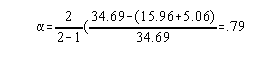
To determine the concurrent validity of the TTC test scores the point biserial correlation coefficient is calculated:
Note: Since the mean for the experts was entered first in the numerator the measures are considered inversely related and so the result of -.83 reflects good concurrent validity for the TTC scores.
Predictive validity is assessed when you want to know whether TTC scores can be used to predict performance on some other variable. The variable your are trying to predict (y) can be called the criterion measure. To assess predictive validity you see how strong the relationship is between your TTC scores and what you are trying to predict. This is done by correlating your TTC scores (x) with measures of the variable you are trying to predict (y). The correlation coefficient used depends on the type of variable the criterion is. The PPMC coefficient is the most common statistic employed in this situation though it is possible to encounter situations requiring the point biserial correlation.
Steps:
For example, assume the scores below came from administration of a TTC test with a success criterion of 3 and measures from another variable (where high score good) to be predicted by the TTC test scores.
| TTC test score | Variable to Predict |
| 11 | 4 |
| 4 | 8 |
| 15 | 4 |
| 3 | 9 |
| 7 | 8 |
| 13 | 6 |
| 8 | 7 |
To determine predictive validity for the TTC scores you calculate the Pearson Product Moment Correlation coefficient and find it to be -.89 so the TTC test scores can be considered to have good predictive validity.
When the purpose of a TTC test is to classify people as masters/non-masters based on one cut score, traditional techniques for estimating reliability and validity do not apply. Data, and subsequent classifications, from a TTC mastery test are valid when relevant, and when they produce correct and consistent classifications of individuals.
Following administration of a TTC test, mastery classifications are made based on a predetermined cut score. Since a low score is good for TTC tests, those scoring below the cut score are masters and those above, non-masters.
Following classification of individuals, the process of estimating the validity of the classificaitons is identical to that involved with any mastery test.
Determined by gathering qualitative evidence that the test measures the fundamental skills needed for entrance, exit, or classification purposes.
There is no statistic to calculate. Evidence is qualitative.
In this context validity is defined as the correct classification of people into mastery states. The most common technique then for assessing the concurrent validity of a TTC mastery test is to examine the test's sensitivity to instruction. That is, if TTC mastery test classifications are valid, an instructed group should be classified as masters and an uninstructed group non-masters when they take the test.
Steps:
| Criterion Classification | |||||
| Master | Non-Master | ||||
| Master | a | b | |||
| TTC Test Classification | |||||
| Non-Master | c | d |
a. Internal consistency
b. Stability
a. Internal consistency
b. Stability
a. Internal consistency
b. Stability
a. Internal consistency
b. Stability
As a test administrator it is important to identify and eliminate as many sources of error as possible in order to enhance reliability. To estimate the amount of measurement error present in observed scores, the standard error of estimate (SEM) can be calculated following calculation of a Relibilty coefficient.
![]()
The SEM is a band + you place around a person's observed score that estimates measurement error.
It is possible to have a reliable data that is invalid. Data/information that is valid should also be reliable. However, reliability does not insure validity.
Reliability is typically assessed in one of two ways:
To estimate reliability you need 2 or more scores per person. If a test is given just once the most common way of getting 2 scores per person is to split the test in half - usually by odd/even trials or items.
Once you have 2 comparable scores per person the question is how consistent overall were the scores. The inference here is that if two sets of scores are consistent there likely is little measurement error and so the scores are likely to be accurrate reflections of true scores and so the observed scores are considered reliable.
In the past, reliability has been estimated using the Pearson Product Moment Correlation coefficient. This is not appropriate since (1) the PPMC is meant to show the relationship between two different variables - not consistency of two measures of the same variable, and (2) the PPMC is not sensitive to fluctuations in test scores.
| X1 | X2 | |
| 10 | 18 | |
| 12 | 19 | |
| 15 | 25 | |
| 17 | 27 |
From the two sets of scores above, rx1,x2 = 1.00 but the scores are not consistent so the PPMC has overestimated reliability. The PPMC is an interclass coefficient; what is needed is an intraclass coefficient. Pearson is appropriately used to estimate Validity not Reliability.
The intraclass statistics that can be used are the intraclass R calculated from values in an analysis of variance (ANOVA) table and coefficient alpha. They are equally acceptable though the ANOVA table the Intraclass R is based on conveys additional information unavailable with coefficient alpha.
This way of examining reliability requires that you give the test once to one group then split the test at least in half to get at least two scores per person. From these two or more scores per person an analysis of variance table (ANOVA) is constructed (typically via software). From this table an Intraclass R can be calculated to assess how consistent the two or more measures per person were.
The reason behind using an ANOVA table is that since you expect variability between students but not variability across measures you should be able to estimate reliability by comparing the variances found in an ANOVA table.
Intraclass R formula:

MSB = mean square between (from ANOVA table)
MSe = mean square error = (SSw + SSi )/ dfw
+ dfi when scores come from comparable parts
SSw = sum of squares within (from ANOVA table)
SSi = sum of squares interaction (from ANOVA table)
dfw = degrees of freedom within (from ANOVA table)
dfi = degrees of freedom interaction (from ANOVA table)
| ANOVA | Table | |||||
| Source of Variance | Degrees of Freedom | Sums of Squares | Mean Squares | |||
| Between | N - 1 | Given | SSb/DFb | |||
| Within | k - 1 | Given | SSw/DFw | |||
| Interaction | (N-1)(k-1) | Given | SSi/DFi | |||
| Total | N(k) - 1 |
N = number of students
k = number of scores per student (not the number of trials/items)
Example: Assume the information in the ANOVA table below came from splitting a 50 item cognitive test administered once. To get two scores per person (number minimally needed to examine reliability) the number correct from the odd and even numbered items was recorded.
| Source | df | SS | MS | |||
| Between | 24 | 6800 | 283.33 | |||
| Within | 1 | 450 | 450 | |||
| Interaction | 24 | 3100 | 129.17 | |||
| Total |


This estimate of reliability is for a test half as long (25 items) as the one administered. Since test length affects reliability this estimate is inaccurate - since the intention was to determine the reliability of scores from the 50 item test - one more step needs to be taken. That is, use the Spearman-Brown Prophecy formula.

Note: Any time test length has been altered or you consider altering it, the spearman-brown formula can be used to estimate what reliability will be provided the items/trials added or deleted are similar to the rest of the test.
For this example, since test length was split in half, m = 2.

This is the estimate of the reliability of scores from the full length test.
The Cronbach's Alpha statistic can be used to estimate the reliability of data under conditions when you have two or more comparable scores per person. These multiple scores per person can come from splits of a test administered once (internal consistency) or they can come from multiple administrations of a test (stability).
Once you have 2 scores per person the question is how consistent overall were the scores. The inference here is that if two sets of scores are consistent there likely is little measurement error and so the scores are likely to be accurrate reflections of true scores and so the observed scores are considered reliable.
Example: Consider a 60 second sit up test administered only once. To get two scores per person you record the number of sit ups completed in the first 30 seconds and the number completed in the second 30 seconds.
| x30 | x30 | Total | ||
| 15 | 18 | 33 | ||
| 26 | 22 | 48 | ||
| 20 | 23 | 43 | ||
| 18 | 18 | 36 | ||
| 25 | 21 | 46 | ||
| 26 | 24 | 50 | ||
| 20 | 19 | 39 |
1. Get the standard deviations for each column
2. Square the standard deviations
3. Use coefficient alpha

Sxt = standard deviation of the
total column (created by you)
Sp = standard deviations of the two or more measures per
student
4. Since test length directly influences reliability it is necessary to boost this reliability coefficient since it tells you only the reliability of a test half as long (30 seconds) as the one you gave yet you set out to establish the reliability of the 60 second test. So, the statistic to help out is called the Spearman-Brown Prophecy formula. It can be employed any time you manipulate test length or want to hypothesize what would happen to reliability if test length were . . . The formula is:
Where m is the amount you wish to boost (or diminish) test length. In this case, since you split the test in half m will be 2 to boost reliability back up to the full length test. So, for the example above the reliability of the full length test is determined by:

Reminder:
As a test administrator it is important to identify and eliminate as many sources of error as possible in order to enhance reliability. To estimate the amount of measurement error present in observed scores, the standard error of estimate (SEM) can be calculated following calculation of a Relibilty coefficient.
![]()
The SEM is a band + you place around a person's observed score that estimates measurement error.
Important Note:
The standard deviation to be used in the SEM formula above is the standard deviation of the total column. The reason is you want a standard deviation that reflects the spread of scores on the full length test.
![]()
Interpretation:
An estimate of measurement error is interpreted relative to the standard deviation of observed scores. The smaller the SEM relative to the standard deviation the more accurate the measures are.
This way of examining reliability requires that you give the test at least twice to one group to get at least two scores per person. From these two or more scores per person an analysis of variance table (ANOVA) is constructed (typically via software). From this table an Intraclass R can be calculated to assess how consistent the two or more measures per person were.
The reason behind using an ANOVA table is that since you expect variability between students but not variability across measures you should be able to estimate reliability by comparing the variances found in an ANOVA table.
Intraclass R formula:
MSB = mean square between (from ANOVA table)
MSe = mean square error = (SSw + SSi )/ dfw
+ dfi
SSw = sum of squares within (from ANOVA table)
SSi = sum of squares interaction (from ANOVA table)
dfw = degrees of freedom within (from ANOVA table)
dfi = degrees of freedom interaction (from ANOVA table)
| ANOVA | Table | |||||
| Source of Variance | Degrees of Freedom | Sums of Squares | Mean Squares | |||
| Between | N - 1 | Given | SSb/DFb | |||
| Within | k - 1 | Given | SSw/DFw | |||
| Interaction | (N-1)(k-1) | Given | SSi/DFi | |||
| Total | N(k) - 1 |
N = number of students
k = number of scores per student (not the number of trials/items)
Assume a test has been given twice and from the 2 scores per person the following ANOVA table is constructed.
| ANOVA | Table | |||||
| Source | df | SS | MS | |||
| Between | 20 | 4000 | 200 | |||
| Within | 1 | 500 | 500 | |||
| Interaction | 20 | 1000 | 50 | |||
| Total |


This way of looking at reliability requires that you give the whole test twice to one group. If the measures are reliable they will be stable over the time between the two administrations and scores will be fairly consistent across the group (provided no significant changes take place between administrations).
Example: Consider a 60 second sit up test administered twice:
| Day 1 | Day 2 | Total | ||
| 52 | 50 | 102 | ||
| 41 | 43 | 84 | ||
| 40 | 38 | 78 | ||
| 34 | 36 | 70 | ||
| 38 | 40 | 78 | ||
| 40 | 42 | 82 |
1. Get the standard deviations for each column
2. Square the standard deviations
3. Use coefficient alpha
![]()
Reminder:
As a test administrator it is important to identify and eliminate as many sources of error as possible in order to enhance reliability. To estimate the amount of measurement error present in observed scores, the standard error of estimate (SEM) can be calculated following calculation of a Relibilty coefficient.
![]()
The SEM is a band + you place around a person's observed score that estimates measurement error.
Important Note:
The standard deviation to be used in the SEM formula above is the standard deviation of an average of the two (or more) scores per person. The reason is you want a standard deviation that reflects the spread of scores on one administration of the test. When you have two or more full length test scores per person, the best estimate of their ability is an average.
| Day 1 | Day 2 | Average | ||
| 52 | 50 | 51 | ||
| 41 | 43 | 42 | ||
| 40 | 38 | 39 | ||
| 34 | 36 | 35 | ||
| 38 | 40 | 39 | ||
| 40 | 42 | 41 |

Note: An estimate of measurement error is interpreted relative to the standard deviation of observed scores. The smaller the SEM relative to the standard deviation the more accurate the measures are.
Reliability is now defined as the accurate (determined by examining consistency) classification of people into mastery states. Again the two perspectives from which reliability can be examined are internal consistency and stability. A mastery test's scores and subsequent classifications based on a cut score are reliable if classifications are consistent over time (stability) or the probability of consistent classification is high (internal consistency).
| Mastery Re-test Classification | |||||
| Master | Non-Master | ||||
| Master | a | b | |||
| Mastery Test Classification | |||||
| Non-Master | c | d |
For example, assume the scores below were from a mastery skills test and the cut score used was 6.
| Test Score | Test Classification | Re-test Score | Re-test Classification | |||
| 12 | (M) | 8 | (M) | |||
| 6 | (M) | 4 | (NM) | |||
| 5 | (NM) | 5 | (NM) | |||
| 4 | (NM) | 6 | (M) | |||
| 7 | (M) | 9 | (M) | |||
| 8 | (M) | 10 | (M) |
| Re-test | |||||
| Master | Non-Master | ||||
| Master | 3 | 1 | |||
| Test | |||||
| Non-Master | 1 | 1 |
Turning the counts above into proportions:
| Re-test | |||||
| Master | Non-Master | ||||
| Master | .50 | .17 | |||
| Test | |||||
| Non-Master | .17 | .17 |
So, the proportion of agreement is: .50 + .17 = .67 meaning that 67% of the classifications made across two administrations of this mastery test were in agreement.
Kappa: This statistic, though fairly unstable when group size small, can take chance into account. In a research setting it is best to always report both Kappa and the Proportion of Agreement. In other cases if you want to report just one, report the Proportion of Agreement. It is easily understood and does give information on stability.
Steps:

Example:
| Re-test | |||||
| Master | Non-Master | ||||
| Master | 5 | 0 | |||
| Test | |||||
| Non-Master | 1 | 2 |
In the example above, the chance component would be:
The proportion of agreement would be
Pag = .63 +.25 = .88
Calculate Kappa

Using the data above, Kappa would be:

A trials-to-criterion test is one where a success criterion (Rc) is set (number of successful attempts to be accumulated) and examinees continue testing until they reach that set criterion. The test score then is the number of trials taken to reach the criterion and a low score reflects good performance.
Or, if you want to express performance as a proportion you can calculate:
p = Rc-1/T-1
where
p = test score expressed as a proportion (on a scale of 0 to 1) - high score is good
Rc = success criterion
T = number of trials taken
Reliability in this context is related to the accuracy of the TTC test scores. Again minimizing measurement error is the key to enhancing reliability. The statistics available for estimating reliabilty include the Intraclass R, Coefficient Alpha, and UEV (for internal consistency only).

To estimate the reliability of scores from a TTC skills test administered once using the Intraclass R, you make use of the multiple scores per person produced when administering a TTC test and from those scores construct an ANOVA table from which you calculate the Intraclass R.
Intraclass R formula:
MSB = mean square between (from ANOVA table)
MSe = mean square error = (SSw + SSi )/ dfw
+ dfi )
SSw = sum of squares within (from ANOVA table)
SSi = sum of squares interaction (from ANOVA table)
dfw = degrees of freedom within (from ANOVA table)
dfi = degrees of freedom interaction (from ANOVA table)
| ANOVA | Table | |||||
| Source of Variance | Degrees of Freedom | Sums of Squares | Mean Squares | |||
| Between | N - 1 | Given | SSb/DFb | |||
| Within | k - 1 | Given | SSw/DFw | |||
| Interaction | (N-1)(k-1) | Given | SSi/DFi | |||
| Total | N(k) - 1 |
N = number of students
k = number of scores per student (in this case it is the value of the success
criterion)
Example: Assume the information in the ANOVA table below came from a TTC test administered once with a success criterion of 5.
| Source | df | SS | MS | |||
| Between | 25 | 7075 | 283 | |||
| Within | 4 | 300 | 75 | |||
| Interaction | 100 | 9000 | 90 | |||
| Total |


To estimate the reliability of scores from a TTC skills test administered once using UEV you work with the TTC test scores' mean and standard deviation.
For example, assume the information below came from a group of 30 who took a TTC badminton serve test where a success criterion of 6 was used.
Mean = 16
Standard Deviation = 10

To estimate the reliability of scores from a TTC skills test administered once using coefficient alpha you make use of the multiple scores per person produced when administering a TTC test and examine the consistency of those scores.
For example, assume the scores below came from a TTC skills test administered once with a success criterion of 4. A zero represents an unsuccessful attempt at the skill and a one a successful attempt. For every student, trials continue to be taken until 4 success have been accumulated. Test score then is the number of trials taken to reach the success criterion of 4.
| Student | trials to 1st success | Trials to 2nd success | Trials to 3rd success | Trials to 4th Success | TTC test Score | |||||
| 1 | 0001 | 00001 | 00001 | 00001 | 19 | |||||
| 2 | 01 | 001 | 1 | 01 | 8 | |||||
| 3 | 1 | 1 | 1 | 1 | 4 | |||||
| 4 | 001 | 01 | 0001 | 001 | 12 | |||||
| 5 | 1 | 01 | 1 | 1 | 5 | |||||
| 6 | 0001 | 001 | 1 | 001 | 11 | |||||
| 7 | 1 | 1 | 001 | 01 | 7 | |||||
| 8 | 01 | 01 | 001 | 01 | 9 |

Reminder:
As a test administrator it is important to identify and eliminate as many sources of error as possible in order to enhance reliability. To estimate the amount of measurement error present in observed scores, the standard error of estimate (SEM) can be calculated following calculation of a Relibilty coefficient.
![]()
The SEM is a band + you place around a person's observed score that estimates measurement error.
Important Note:
The standard deviation to be used in the SEM formula above is the standard deviation of the TTC test score column. The reason is you want a standard deviation that reflects the spread of scores on the full length TTC test.
![]()
Interpretation:
An estimate of measurement error is interpreted relative to the standard deviation of observed scores. The smaller the SEM relative to the standard deviation the more accurate the measures are.
This way of examining reliability requires that you give the TTC test at least twice to one group to get at least two scores per person. From these two or more scores per person an analysis of variance table (ANOVA) is constructed (typically via software). From this table an Intraclass R can be calculated to assess how consistent the two or more measures per person were.
For example, assume you administered a TTC test with a success criterion of 6 to a group then retested them three more times. From these four scores per person you construct an ANOVA table from which you calculate the Intraclass R statistic to estimate reliability.
| Source | df | SS | MS | |||
| Between | 27 | 6870 | 254.44 | |||
| Within | 3 | 1200 | 400 | |||
| Interaction | 81 | 9340 | 115.31 | |||
| Total |

To estimate the reliability of scores from a TTC skills test administered at least twice using coefficient alpha you use the TTC test score from each administration of the TTC test for each individual.
For example, assume you administered a TTC test with a success criterion of 5 to a group then retested them two more times. From these three scores per person you assess reliability by examining the consistency across the 3 sets of scores using coefficient alpha.
| TTC Test | TTC Re-test | TTC Re-test | Total | |||
| 18 | 19 | 17 | 54 | |||
| 12 | 15 | 13 | 40 | |||
| 7 | 10 | 8 | 25 | |||
| 10 | 9 | 9 | 28 | |||
| 12 | 10 | 10 | 32 | |||
| 15 | 14 | 13 | 42 |

Reminder:
As a test administrator it is important to identify and eliminate as many sources of error as possible in order to enhance reliability. To estimate the amount of measurement error present in observed scores, the standard error of estimate (SEM) can be calculated following calculation of a Relibilty coefficient.
![]()
The SEM is a band + you place around a person's observed score that estimates measurement error.
Important Note:
The standard deviation to be used in the SEM formula above is the standard deviation of an average of the two multiple scores per person. The reason is you want a standard deviation that reflects the spread of scores on one administration of the test. When you have two or more full length test scores per person, the best estimate of their ability is an average.
| Test | Re-test | Re-test | Average | |||
| 18 | 19 | 17 | 18 | |||
| 12 | 15 | 13 | 13.33 | |||
| 7 | 10 | 8 | 8.33 | |||
| 10 | 9 | 9 | 9.33 | |||
| 12 | 10 | 10 | 10.67 | |||
| 15 | 14 | 13 | 14 |
![]()
Note: An estimate of measurement error is interpreted relative to the standard deviation of observed scores. The smaller the SEM relative to the standard deviation the more accurate the measures are.
A student's TTC score is now converted to a classification (master or non-master) based on a predetermined cut score. As in any other mastery testing framework determining a good cut score is the most difficult element. One approach however, is to determine (from a philosophical perspective) what you believe the probability of success should be for a master then convert that probability to a cut score. The conversion is done by:
TTC score = R/p
R = success criterion
p = probability of success expressed as a proportion
For example, assume the probability of success you would expect from a master of some skill is .65 and the success criterion you want to use in your TTC test is 7. The TTC cut score you would use to classify examinees as masters or non-masters would be:
TTC score = 7/.65 = 10.77
So, TTC cut score = 10.77. Remember that a low score is good on a TTC test. Therefore individuals with a TTC score below 10.77 are classified as masters and those above 10.77 are classified as non-masters.
Methods
| TTC Mastery Re-test |
|||||
| Master | Non-Master | ||||
| Master | a | b | |||
| TTC Mastery Test Classification | |||||
| Non-Master | c | d |
Kappa: This statistic, though fairly unstable when group size small, can take chance into account. In a research setting it is best to always report both Kappa and the Proportion of Agreement. In other cases if you want to report just one, report the Proportion of Agreement. It is easily understood and does give information on stability.
Steps:
6. Calculate Kappa
Whenever measures have a strong subjective component to them it is essential to examine objectivity. Subjectivity itself is a source of measurement error and so affects reliability and validity. Therefore, objectivity is a matter of determining the accuracy of measures by examining consistency across multiple observations (multiple judges on one ocasion or repeated measures over time from one evaluator) that typically involve the use of rating scales.
To examine objectivity you need to have either multiple evaluators assessing performance/knowledge on one occasion, or one evaluator assessing the same performance (videotaped)/knowledge twice. The two or more measures per examinee collected are then used to construct an ANOVA table from which the Intraclass R can be calculated.
If the measures (typically from a rating scale) are objective they will be consistent across the two or more measures per examinee.
Example: Consider a skills test assessing Tennis serve technique. One qualified observer scores each person in a group using a rating scale that assesses the execution of the tennis serve. That same observer rates the videotaped serves from each person a second time without reference to the first ratings. Objectivity is then estimated by using these two scores per examinee to construct an ANOVA table and calculate the Intraclass R.
| Source | df | SS | MS | |||
| Between | 29 | 4350 | 150 | |||
| Within | 1 | 40 | 40 | |||
| Interaction | 29 | 1450 | 50 | |||
| Total |


This way of examining objectivity requires that you have either multiple evaluators assessing performance/knowledge on one occaision, or one evaluator assessing the same performance (videotaped)/knoledge twice. If the measures (typically from a rating scale) are objective they will be consistent across the two or more measures per examinee.
Example: Consider a skills test assessing cartwheel technique. Three qualified observers score each person in a group using a rating scale that assesses the execution of the components of a cartwheel. Objectivity can then be estimated using coefficient alpha.
| Student | Judge 1 | Judge 2 | Judge 3 | Total | ||||
| 1 | 12 | 10 | 8 | 30 | ||||
| 2 | 8 | 10 | 11 | 29 | ||||
| 3 | 3 | 4 | 5 | 12 | ||||
| 4 | 14 | 10 | 11 | 35 | ||||
| 5 | 10 | 10 | 12 | 32 | ||||
| 6 | 8 | 8 | 9 | 25 | ||||
| 7 | 7 | 8 | 9 | 24 | ||||
| 8 | 10 | 10 | 9 | 29 | ||||
| 9 | 12 | 10 | 10 | 32 |

Reminder:
As a test administrator it is important to identify and eliminate as many sources of error as possible in order to enhance reliability. To estimate the amount of measurement error present in observed scores, the standard error of estimate (SEM) can be calculated following calculation of an objectivity coefficient.
![]()
The SEM is a band + you place around a person's observed score that estimates measurement error.
Important Note:
The standard deviation to be used in the SEM formula above is the standard deviation of an average of the multiple scores per person. The reason is you want a standard deviation that reflects the spread of scores for the best measure of ability. When you have two or more test scores per person, the best estimate of their ability is an average.
| Student | Judge 1 | Judge 2 | Judge 3 | Average | ||||
| 1 | 12 | 10 | 8 | 10 | ||||
| 2 | 8 | 10 | 11 | 9.67 | ||||
| 3 | 3 | 4 | 5 | 4 | ||||
| 4 | 14 | 10 | 11 | 11.67 | ||||
| 5 | 10 | 10 | 12 | 10.67 | ||||
| 6 | 8 | 8 | 9 | 8.33 | ||||
| 7 | 7 | 8 | 9 | 8 | ||||
| 8 | 10 | 10 | 9 | 9.67 | ||||
| 9 | 12 | 10 | 10 | 10.67 |
![]()
Note: An estimate of measurement error is interpreted relative to the standard deviation of observed scores. The smaller the SEM relative to the standard deviation the more accurate the measures are.